

In geophysical catastrophe modelling, the Beta distribution is the most popular probability distribution used to describe uncertainty in loss severity. The distribution is a continuous two-parameter function bounded by values of zero and unity.
The PDF of the Beta distribution is a function of its two shape parameters A and B:

β(A,B) simply normalises the distribution and is given by

where Γ is the Gamma function.
The expected loss of the distribution is given by:

and its variance by:
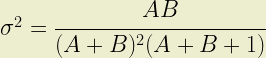
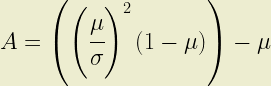
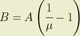
In catastrophe modelling applications it is normal to want to derive the shape parameters from an expected loss and its standard deviation. A little work shows us that
Note, the distribution is evaluated on values of x bounded by 0 and 1. In catastrophe modelling applications, the expected loss μ is represented by the ratio of the expected loss to the sum insured (or limit, or “exposed value”)