April 2017 – Life, the universe and cat modelling

On Beta Distributions (Part 3)

This post explores the shape of Beta distributions typically used to represent original (“ground up” or damage) loss distributions in commercial catastrophe models.

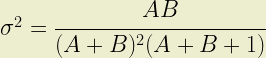
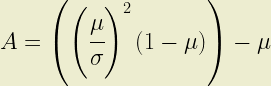
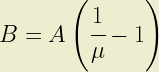
The shape parameters of the Beta distribution, A and B, must be both positive and real. This places some constraints on the values of expected loss (µ) and standard deviation (σ) which can be represented with a beta distribution. Part 1 describes how the shape parameter A can be expressed as a function of µ and σ. Constraining A > 0 it is simple to show that:

$C \ \textless \ \sqrt{\cfrac{1-\mu}{\mu}}$

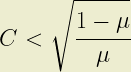
where C represents the coefficient of variation; the ratio of standard deviation to expected loss. It follows that the second shape parameter, B, also satisfies the constraint because 0 < µ < 1 is always true.

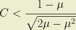
The same approach shows that A < 1 results when:

$C \ \textgreater \ \sqrt{\cfrac{1-\mu}{1+\mu}}$

and A > 1 when:

$C \ \textless \ \sqrt{\cfrac{1-\mu}{1+\mu}}$

(Note that C is constrained to be <1 whenever A>1)

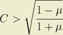
Similarly, it is simple to show that B < 1 where:

$A \ \textgreater \ \cfrac{\mu}{1-\mu}$

and therefore where:

$C \ \textgreater \ \cfrac{1-\mu}{\sqrt{2\mu - \mu^2}}$

Finally, B > 1 where:

$C \ \textless \ \cfrac{1-\mu}{\sqrt{2\mu - \mu^2}}$

Plotting contours of these C(µ) relationships results in the following graph:

1. Linear-log contour plot of C(µ) for shape parameters near 0 and 1

These contours demark the four basic shapes of the beta distribution as described in Part 2. Replotting this graph as linear-log distorts the plot but allows the four basic shapes of the distribution to be shown within these contours:

2. Log-linear plot of C(µ) contours demarking the 4 basic shapes of the beta distribution

Unsurprisingly this blog does not itself hold a licence for any of the commercial vendor models, so data from the model vendors will not be shown. Nonetheless, any reader with access to a vendor model is invited to explore location- or risk-level C(µ) relationships in their models. This is easy to do: simply report expected loss and standard deviation per event for a single, geocoded location referencing a single vulnerability function.

An empirical observation is that original damage relationships never fall in the range where the beta distribution B parameter takes a value <1. This appears to be true for all perils, all geographies and all vendors (even those that do not model original loss severity with a beta distribution).

Part 2 established that (1) the beta distribution can only approximate total losses and (2) this only occurs when the B shape parameter is less than unity. In other words, even at location level, those commercial models using beta distributions don’t even approximate total loss to a location.

Again, this bears repeating. Those models which use a beta distribution to model loss severity do not consider total loss. Moreover, they do not even approximate total loss.

(It is also worth noting that – even under perfect correlation of standard deviations – C cannot increase as location loss distributions are combined. Therefore, it is not possible for any aggregate loss distribution approximate total loss).

On Beta Distributions (Part 2)

Beta distributions appear everywhere in catastrophe modelling. At least, they appear more often than not when a vendor is trying to represent uncertainty in loss severity. This is odd, considering how rarely this distribution is used in other actuarial or engineering disciplines. Nonetheless, all of the major catastrophe model vendors use Beta distributions somewhere in their financial engines; and one or two even use the Beta distribution exclusively.

The most common justification for using the Beta distribution is its ability to assume many forms. It is, of course, reasonable to wonder whether a distribution capable of assuming so many different forms can represent any physical reality. There is also a more pragmatic explanation; a distribution naturally bounded by zero and unity doesn’t need artificial truncation to avoid (a) negative loss or (b) losses greater than the sum insured.

The PDF has four basic shapes, depending on the values of the (positive, real) shape parameters A and B described in Part 1. The following four figures show the basic shape of the distribution for the four cases where each parameter can take values less than or greater than unity.

(Note, in the case of either shape parameter taking a value of 1 a power law distribution results. If both shape parameters are unity, the PDF is also unity for all values of x.)

The first thing to observe is that in all cases, the probability of both zero loss and total loss is zero. In other words, wherever a Beta distribution is being used to model loss severity, neither zero loss nor total loss are considered. This becomes evident when the PDF formula in Part 1 is examined.

This is worth repeating. Whenever a Beta distribution is used to represent loss severity, total loss is not possible. Similarly, there is no possibility of zero loss. This is not unreasonable when modelling losses to aggregates. However, this is – at very best – questionable when modelling losses to individual properties (i.e. using “detailed” data).

It could be argued that cases 1 and 2 appear to make a reasonable approximation of representing zero loss; and cases 1 and 3 appear to do the same for total loss. It is therefore instructive to look at the circumstances under which the original (“ground up” or “damage”) distribution could assume each of these shapes. This will be explored in the next post on Beta distributions.

(Note, the application of non-proportional financial terms such as excess points and first loss limits introduces more parameters and further complicates the general description made here. For this reason original loss distributions will be investigated)

On Beta Distributions (Part 1)

In geophysical catastrophe modelling, the Beta distribution is the most popular probability distribution used to describe uncertainty in loss severity. The distribution is a continuous two-parameter function bounded by values of zero and unity.

The PDF of the Beta distribution is a function of its two shape parameters A and B:

$P(x) = \beta(A,B)x^{A-1}(1-x)^{B-1}$

β(A,B) simply normalises the distribution and is given by

$\beta(A,B) = \cfrac{\Gamma(A+B)}{\Gamma(A)\Gamma(B)}$

where Γ is the Gamma function.

The expected loss of the distribution is given by:

$\mu = \cfrac{A}{A+B}$

and its variance by:

$\sigma^2 = \cfrac{AB}{(A+B)^2(A+B+1)}$

In catastrophe modelling applications it is normal to want to derive the shape parameters from an expected loss and its standard deviation. A little work shows us that

$A = \left(\left(\cfrac{\mu}{\sigma}\right)^2\left(1-\mu\right)\right)-\mu$

$B = A\left(\cfrac{1}{\mu}-1\right)$

Note, the distribution is evaluated on values of x bounded by 0 and 1. In catastrophe modelling applications, the expected loss μ is represented by the ratio of the expected loss to the sum insured (or limit, or “exposed value”)

València 2015

This post relates to events taking place almost 18 months before this blog even existed. The bitterness that followed has never really gone away so this is still, in some small way, relevant to MotoGP today. This first post will cover a quick analysis done shortly after València 2015.

First a quick recap. At the penultimate round of the 2015 championship Valentino Rossi accused Marc Márquez of having “played” with the other riders during the previous round at Phillip Island. He went on to say that he thought Márquez did this to support Jorge Lorenzo’s world championship. Márquez denied this and the two riders clashed during the race. This earned Rossi three penalty points; relegating him to the back of the grid for the championship decider in València. Lorenzo won the final race and with it the championship. Then the real bitterness started, as Rossi accused Márquez of protecting Lorenzo in the race to ensure his championship victory.

The accusations generated plenty of opinion but not much actual analysis. Here are my observations, based on the lap times published on motogp.com.

The first figure shows lap times for the top four riders at Phillip Island. The second figure simplifies this by showing times for the podium contenders over the last four laps. It is pretty clear to see that Márquez won the race by riding the fastest lap of the race on the final lap. This fits the narrative at the time: Márquez having gone all out for glory with an amazing final lap. We can also see that his penultimate lap was quicker than the other podium contenders and that they all slowed – while he went quicker – on the final lap.

Márquez’s final lap was 0.38s quicker than his penultimate lap, which was itself a good lap. There’s not much point comparing the last lap to a trended average lap time because his lap times were so inconsistent. In fact, we see a lot of inconsistency in lap times for the top four over the race. This is understandable given the amount of overtaking in the race.

The next two graphs show the same information for the top four riders at the València round. Once again we see that Márquez has a great final lap (0.49s quicker than his penultimate lap). Crucially we also see that both Lorenzo and Pedrosa are also quicker on their final laps, each by 0.24s.

It’s hard to see anything in the lap times to indicate that Márquez wasn’t really trying at València. It looks very much like he’s trying to win the race, just as he did at Phillip Island. Admittedly the teams and riders have access to more data than this but what could they possibly have that would contradict the obvious conclusion from lap times?

Welcome

This is where I blog about what I really think. It will mostly be about cat modelling